Multiperiod hledger-Style Reports in beancount: Pivoting a Table
I am using plain text accounting tools like hledger and beancount alongside KMyMoney to track my financial transactions and to produce summary reports about income and expenses. If you’ve ever used hledger, you might like its ability to produce nice reports. One of the reports’ feature is the table structure, where rows are accounts and columns are weeks, months, quarters or years. Looking at earnings and spendings as a function of time can give you more insights about your finances.
However, if you are using beancount, this feature is not yet supported in the command line interface. You need to use fava, an awesome web-interface for beancount, which has a graph drawing capability as described in this tutorial. fava is not ideal and sometimes you might need more custom reports than the ones available in fava.
Problem Statement
Suppose that you have an example beancount journal file and you want to see your income and expenses for every year. This can be accomplished by following BQL-query:
1 2 3 4 5 6 7 8 9 10 |
[johndoe@ArchLinux]% bean-example > example.beancount [johndoe@ArchLinux]% bean-query example.beancount\ "SELECT account,\ YEAR(date) AS year,\ SUM(convert(position, 'USD', date)) AS amount\ WHERE\ account ~ 'Expenses' OR\ account ~ 'Income'\ GROUP BY account, year\ ORDER BY account, year" |
which will generate the following table:
1 2 3 4 5 6 7 8 9 10 11 12 13 |
account year amount ------------------------------------------ ---- ----------------- Expenses:Financial:Commissions 2018 116.35 USD Expenses:Financial:Commissions 2019 125.30 USD Expenses:Financial:Commissions 2020 232.70 USD Expenses:Financial:Fees 2018 48.00 USD Expenses:Financial:Fees 2019 48.00 USD ... Income:US:Hoogle:Salary 2019 -119999.88 USD Income:US:Hoogle:Salary 2020 -124615.26 USD Income:US:Hoogle:Vacation 2018 -130 VACHR Income:US:Hoogle:Vacation 2019 -130 VACHR Income:US:Hoogle:Vacation 2020 -135 VACHR |
“PIVOT BY account, year” would implement the following restructuring of the table by adding time dimension (year):
1 2 3 4 5 6 7 8 9 10 11 12 13 |
account/year 2018 2019 2020 ------------------------------ -------------- -------------- -------------- Expenses:Financial:Commissions 116.35 USD 125.30 USD 232.70 USD Expenses:Financial:Fees 48.00 USD 48.00 USD 48.00 USD Expenses:Food:Coffee 5.49 USD 36.76 USD 43.07 USD Expenses:Food:Groceries 2298.84 USD 2365.05 USD 2291.58 USD Expenses:Food:Restaurant 4064.22 USD 4955.84 USD 4401.07 USD ... Income:US:ETrade:VEA:Dividend 0.00 USD -55.23 USD -138.35 USD Income:US:ETrade:VHT:Dividend -50.90 USD 0.00 USD -175.33 USD Income:US:Hoogle:GroupTermLife -632.32 USD -632.32 USD -656.64 USD Income:US:Hoogle:Match401k -9250.00 USD -9250.00 USD -9250.00 USD Income:US:Hoogle:Salary -119999.88 USD -119999.88 USD -124615.26 USD |
This feature is NOT implemented yet, but there is a way to emulate it using Pandas library.
Exporting beancount Data to Pandas Dataframe
We can dive in into internals of the beancount library and use Python functions to extract raw or processed data:
1 2 3 4 5 6 7 8 9 10 11 12 13 14 15 16 17 18 19 20 21 22 23 24 25 26 27 28 29 30 31 32 33 34 35 |
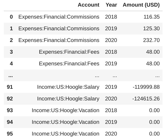
#!/usr/bin/env python # Export beancount raw data to Pandas dataframe from beancount.loader import load_file from beancount.query.query import run_query from beancount.query.numberify import numberify_results import os import pandas as pd import numpy as np # Create an Example beancount Journal File FileName = "example.beancount" if not os.path.isfile(FileName): os.system("bean-example > {}".format(FileName)) # Load an Example beancount Journal File entries, _, opts = load_file(FileName) # Main currency currency = opts["operating_currency"][0] # Executing a BQL Query cols, rows = run_query(entries, opts, "SELECT account, YEAR(date) AS year, SUM(convert(position, '{}', date)) AS amount\ WHERE account ~ 'Expenses'\ OR account ~ 'Income'\ GROUP BY account, year ORDER BY account, year".format(currency) ) cols, rows = numberify_results(cols, rows) # Converting Result Rows to a Pandas Dataframe df = pd.DataFrame(rows, columns=[k[0] for k in cols]) df.rename(columns={"account": "Account", "year":"Year", "amount ({})".format(currency): "Amount ({})".format(currency)}, inplace=True) df = df.astype({"Account": str, "Year": int, "Amount ({})".format(currency): np.float}) print(df[["Account", "Year", "Amount ({})".format(currency)]].fillna(0)) |
will print the following dataframe:
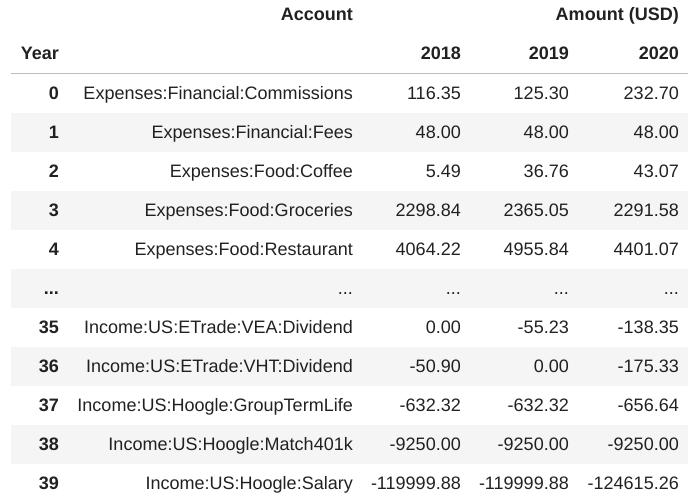
Pivoting the table by year
1 2 3 |
# Pivoting a Table by Year df = df.pivot_table(index="Account", columns=[ 'Year']).fillna(0).reset_index() print(df) |
yields:
Converting account names into multi-level account hierarchy
1 2 3 4 5 6 |
# Creating Multi-Level Accounts n_levels = df["Account"].str.count(":").max() + 1 cols = ["Account_L{}".format(k) for k in range(n_levels)] df[cols] = df["Account"].str.split(':', n_levels - 1, expand=True) df = df.fillna('').drop(columns="Account", level=0).set_index(cols) print(df) |
produces a multi-index dataframe:
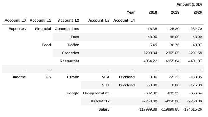
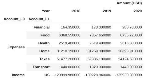
This dataframe can help to produce aggregation at different account levels:
1 2 |
# Aggregation at Different Account Levels print(df.groupby(["Account_L0", "Account_L1"]).sum()) |
You can invert the counter-intuitive negative sign of the “Income” account and plot income (level 0) and expenses (level 0) aggregated at a year interval:
1 2 3 4 5 6 7 8 9 10 11 12 13 14 |
from matplotlib import pyplot as plt font = {'weight' : 'normal', 'size' : 12} plt.rc('font', **font) plt.rcParams["figure.figsize"] = (15, 5) df_L0 = df.groupby(["Account_L0"]).sum() # Invert the sign of the "Income" account. Negative income is counter-intuitive. df_L0.loc["Income"] = -df_L0.loc["Income"] df_L0 = df_L0.transpose().reset_index() df_L0.columns.name = "Account" df_L0.plot.bar(x="Year", y=["Income", "Expenses"], ylabel=df_L0["level_0"][0], rot=0) plt.show() |

Or make a treemap plot of the expenses:
1 2 3 4 5 6 7 8 9 10 11 12 13 14 15 16 17 18 19 20 21 22 23 24 25 |
import squarify df_L1 = df.groupby(["Account_L0", "Account_L1"]).sum() tot = df_L1.sum(axis=1).to_frame() # Treemap Plot of Expenses data = tot.loc["Expenses"].sort_values(by=0, ascending=False) values = data.values labels = data.index width = 1 height = 0.5 values_norm = squarify.normalize_sizes(values, width, height) rects = squarify.squarify(values_norm, 0, 0, width, height) fig = plt.figure(figsize=(10, 10)) fig.suptitle('Expenses', x=0.5, y=0.55, fontsize=16) axes = [fig.add_axes([rect['x'], rect['y'], rect['dx'], rect['dy'], ]) for rect in rects] for ax, txt, color in zip(axes, labels, plt.cm.Pastel1.colors): ax.text(0.5, 0.5, txt, horizontalalignment='center', verticalalignment='center') ax.set_yticks([]) ax.set_xticks([]) ax.set_facecolor(color) plt.show() |

Aggregation at Month and Quarter Levels
Aggregation of transaction amounts at different time intervals (months, quarters) requires a different BQL query and a bit more playing with pandas.DatetimeIndex. The scripts and details are in the git repository.


Summary
- “Pivot by” functionality can be implemented using Pandas library.
- Negative sign of the quantities in the “Income” account can be fixed easily and graphs/figures similar to fava’s ones can be plotted using matplotlib. In fava, negative sign of the income category has not been fixed yet.
- Aggregation at different account levels can be done easily using mutli-index dataframes in Pandas.
- The source code is available in this git repository.
References
“Beancount Query Languge” by Martin Blais
“Managing my personal finances with beancount” by Alex Johnstone
Comments powered by Disqus.